Oil Price History and Analysis

Oil Price History and Analysis (Updating)	A discussion of crude oil prices, the relationship between prices and rig count and the outlook for the future of the petroleum industry.
Introduction Crude oil prices behave much as any other commodity with wide price swings in times of shortage or oversupply. The crude oil price cycle may extend over several years responding to changes in demand as well as OPEC and non-OPEC supply. The U.S. petroleum industry's price has been heavily regulated through production or price controls throughout much of the twentieth century. In the post World War II era U.S. oil prices at the wellhead averaged $24.98 per barrel adjusted for inflation to 2007 dollars. In the absence of price controls the U.S. price would have tracked the world price averaging $27.00. Over the same post war period the median for the domestic and the adjusted world price of crude oil was $19.04 in 2007 prices. That means that only fifty percent of the time from 1947 to 2007 have oil prices exceeded $19.04 per barrel. (See note in box on right.) Until the March 28, 2000 adoption of the $22-$28 price band for the OPEC basket of crude, oil prices only exceeded $24.00 per barrel in response to war or conflict in the Middle East. With limited spare production capacity OPEC abandoned its price band in 2005 and was powerless to stem a surge in oil prices which was reminiscent of the late 1970s.	Crude Oil Prices 1947 - May, 2008 Click on graph for larger view *World Price - The only very long term price series that exists is the U.S. average wellhead or first purchase price of crude. When discussing long-term price behavior this presents a problem since the U.S. imposed price controls on domestic production from late 1973 to January 1981. In order to present a consistent series and also reflect the difference between international prices and U.S. prices we created a world oil price series that was consistent with the U.S. wellhead price adjusting the wellhead price by adding the difference between the refiners acquisition price of imported crude and the refiners average acquisition price of domestic crude.
The Very Long Term View The very long term view is much the same. Since 1869 US crude oil prices adjusted for inflation have averaged $21.05 per barrel in 2006 dollars compared to $21.66 for world oil prices. Fifty percent of the time prices U.S. and world prices were below the median oil price of $16.71 per barrel. If long term history is a guide, those in the upstream segment of the crude oil industry should structure their business to be able to operate with a profit, below $16.71 per barrel half of the time. The very long term data and the post World War II data suggest a "normal" price far below the current price.	Crude Oil Prices 1869-2007 Click on graph for larger view
The results are dramatically different if only post-1970 data are used. In that case U.S. crude oil prices average $29.06 per barrel and the more relevant world oil price averages $32.23 per barrel. The median oil price for that time period is $26.50 per barrel. If oil prices revert to the mean this period is likely the most appropriate for today's analyst. It follows the peak in U.S. oil production eliminating the effects of the Texas Railroad Commission and is a period when the Seven Sisters were no longer able to dominate oil production and prices. It is an era of far more influence by OPEC oil producers than they had in the past. As we will see in the details below influence over oil prices is not equivalent to control.	Crude Oil Prices 1970-2007 Click on graph for larger view
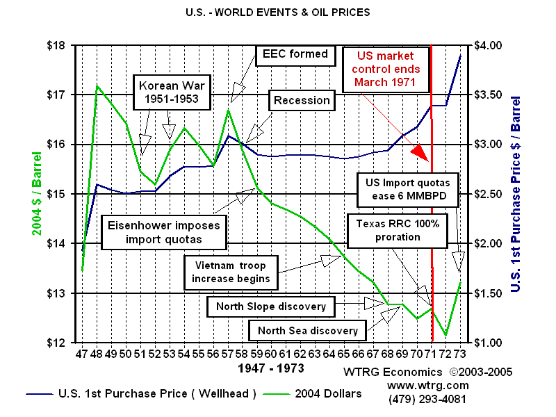
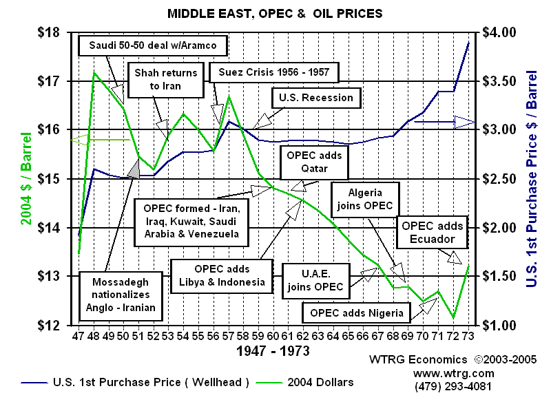
Post World War II Pre Embargo Period Crude Oil prices ranged between $2.50 and $3.00 from 1948 through the end of the 1960s. The price oil rose from $2.50 in 1948 to about $3.00 in 1957. When viewed in 2006 dollars an entirely different story emerges with crude oil prices fluctuating between $17 - $18 during the same period. The apparent 20% price increase just kept up with inflation. From 1958 to 1970 prices were stable at about $3.00 per barrel, but in real terms the price of crude oil declined from above $17 to below $14 per barrel. The decline in the price of crude when adjusted for inflation was amplified for the international producer in 1971 and 1972 by the weakness of the US dollar. OPEC was formed in 1960 with five founding members Iran, Iraq, Kuwait, Saudi Arabia and Venezuela. Two of the representatives at the initial meetings had studied the the Texas Railroad Commission's methods of influencing price through limitations on production. By the end of 1971 six other nations had joined the group: Qatar, Indonesia, Libya, United Arab Emirates, Algeria and Nigeria. From the foundation of the Organization of Petroleum Exporting Countries through 1972 member countries experienced steady decline in the purchasing power of a barrel of oil. Throughout the post war period exporting countries found increasing demand for their crude oil but a 40% decline in the purchasing power of a barrel of oil. In March 1971, the balance of power shifted. That month the Texas Railroad Commission set proration at 100 percent for the first time. This meant that Texas producers were no longer limited in the amount of oil that they could produce. More importantly, it meant that the power to control crude oil prices shifted from the United States (Texas, Oklahoma and Louisiana) to OPEC. Another way to say it is that there was no more spare capacity and therefore no tool to put an upper limit on prices. A little over two years later OPEC would, through the unintended consequence of war, get a glimpse at the extent of its power to influence prices.	World Events and Crude Oil Prices 1947-1973 Click on graph for larger view Middle East, OPEC and Oil Prices 1947-1973 Click on graph for larger view
Middle East Supply Interruptions Yom Kippur War - Arab Oil Embargo In 1972 the price of crude oil was about $3.00 per barrel and by the end of 1974 the price of oil had quadrupled to over $12.00. The Yom Kippur War started with an attack on Israel by Syria and Egypt on October 5, 1973. The United States and many countries in the western world showed support for Israel. As a result of this support several Arab exporting nations imposed an embargo on the countries supporting Israel. While Arab nations curtailed production by 5 million barrels per day (MMBPD) about 1 MMBPD was made up by increased production in other countries. The net loss of 4 MMBPD extended through March of 1974 and represented 7 percent of the free world production. If there was any doubt that the ability to control crude oil prices had passed from the United States to OPEC it was removed during the Arab Oil Embargo. The extreme sensitivity of prices to supply shortages became all too apparent when prices increased 400 percent in six short months. From 1974 to 1978 world crude oil prices were relatively flat ranging from $12.21 per barrel to $13.55 per barrel. When adjusted for inflation the price over that period of time world oil prices were in a period of moderate decline.	U.S. and World Events and Oil Prices 1973-1981 Click on graph for larger view OPEC Oil Production 1973-2007 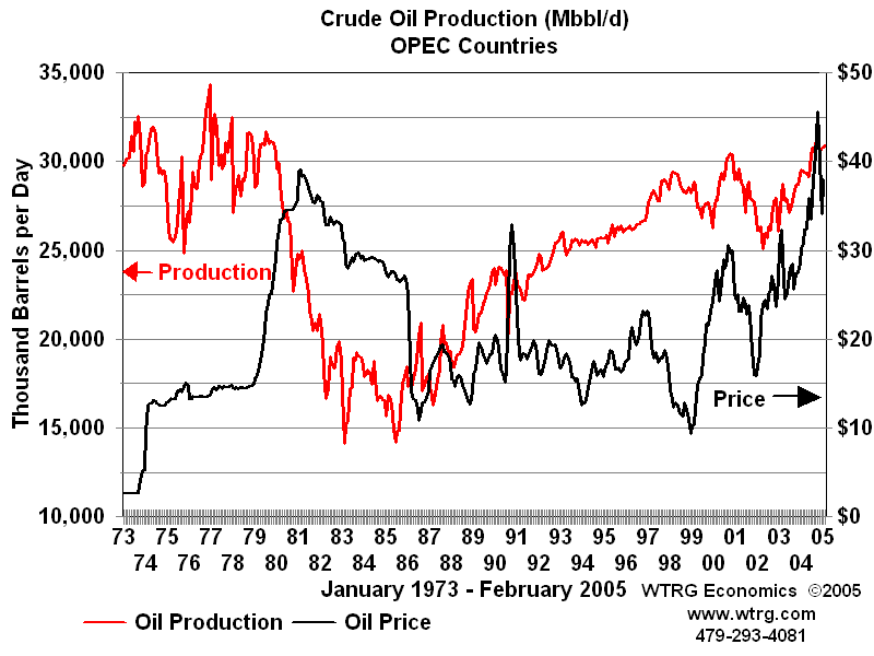Click on graph for larger view
Crises in Iran and Iraq Events in Iran and Iraq led to another round of crude oil price increases in 1979 and 1980. The Iranian revolution resulted in the loss of 2 to 2.5 million barrels per day of oil production between November, 1978 and June, 1979. At one point production almost halted. While the Iranian revolution was the proximate cause of what would be the highest prices in post-WWII history, its impact on prices would have been limited and of relatively short duration had it not been for subsequent events. Shortly after the revolution production was up to 4 million barrels per day. Iran weakened by the revolution was invaded by Iraq in September, 1980. By November the combined production of both countries was only a million barrels per day and 6.5 million barrels per day less than a year before. As a consequence worldwide crude oil production was 10 percent lower than in 1979. The combination of the Iranian revolution and the Iraq-Iran War cause crude oil prices to more than double increasing from from $14 in 1978 to $35 per barrel in 1981. Twenty-six years later Iran's production is only two-thirds of the level reached under the government of Reza Pahlavi, the former Shah of Iran. Iraq's production remains about 1.5 million barrels below its peak before the Iraq-Iran War.	Iran Oil production 1973-2007 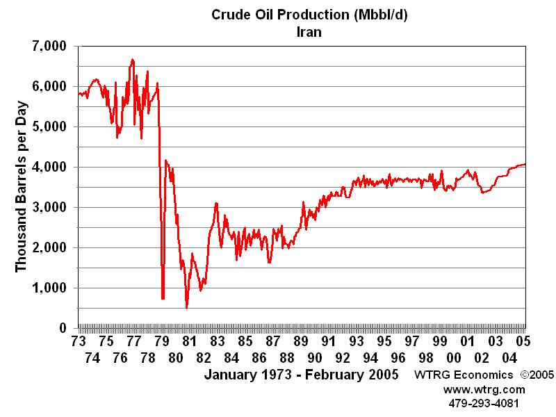Click on graph for larger view Iraq Oil production 1973-2007 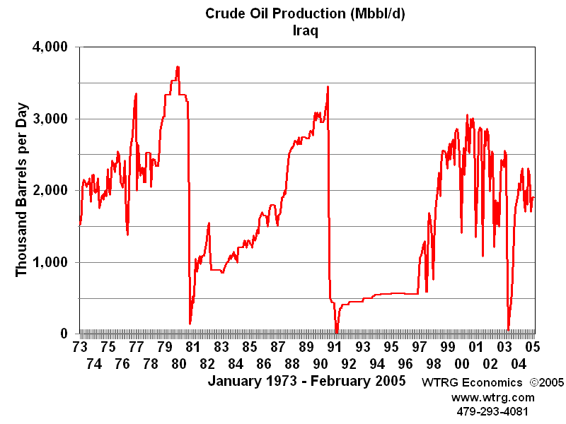Click on graph for larger view
US Oil Price Controls - Bad Policy? The rapid increase in crude prices from 1973 to 1981 would have been much less were it not for United States energy policy during the post Embargo period. The US imposed price controls on domestically produced oil in an attempt to lessen the impact of the 1973-74 price increase. The obvious result of the price controls was that U.S. consumers of crude oil paid about 50 percent more for imports than domestic production and U.S producers received less than world market price. In effect, the domestic petroleum industry was subsidizing the U.s. consumer. Did the policy achieve its goal? In the short term, the recession induced by the 1973-1974 crude oil price rise was less because U.S. consumers faced lower prices than the rest of the world. However, it had other effects as well. In the absence of price controls U.S. exploration and production would certainly have been significantly greater. Higher petroleum prices faced by consumers would have resulted in lower rates of consumption: automobiles would have had higher miles per gallon sooner, homes and commercial buildings would have been better insulated and improvements in industrial energy efficiency would have been greater than they were during this period. As a consequence, the United States would have been less dependent on imports in 1979-1980 and the price increase in response to Iranian and Iraqi supply interruptions would have been significantly less.	US Oil Price Controls 1973-1981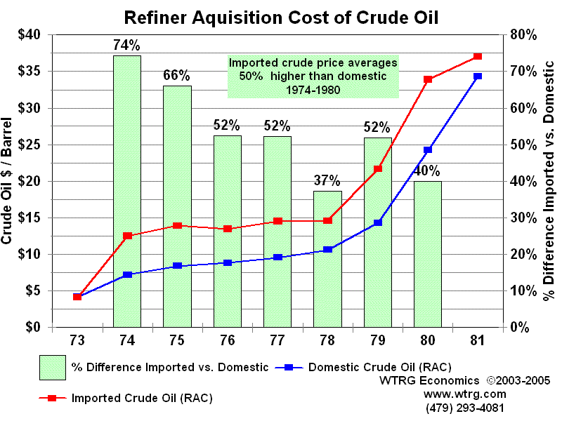 Click on graph for larger view
OPEC's Failure to Control Crude Oil Prices
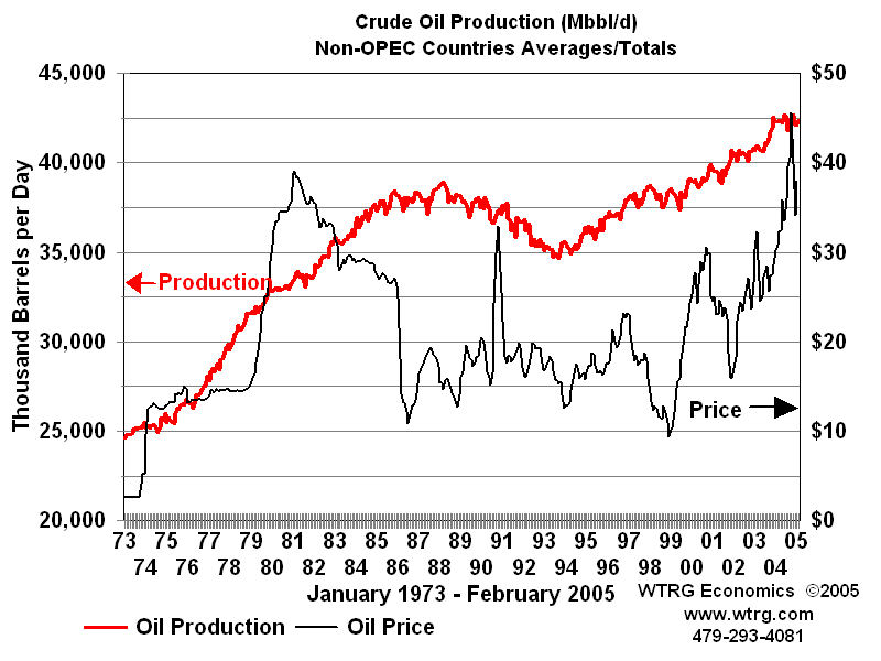
OPEC has seldom been effective at controlling prices. While often referred to as a cartel, OPEC does not satisfy the definition. One of the primary requirements is a mechanism to enforce member quotas. The old joke went something like this. What is the difference between OPEC and the Texas Railroad Commission? OPEC doesn't have any Texas Rangers! The only enforcement mechanism that has ever existed in OPEC was Saudi spare capacity. With enough spare capacity at times to be able to increase production sufficiently to offset the impact of lower prices on its own revenue, Saudi Arabia could enforce discipline by threatening to increase production enough to crash prices. In reality even this was not an OPEC enforcement mechanism unless OPEC's goals coincided with those of Saudi Arabia. During the 1979-1980 period of rapidly increasing prices, Saudi Arabia's oil minister Ahmed Yamani repeatedly warned other members of OPEC that high prices would lead to a reduction in demand. His warnings fell on deaf ears. Surging prices caused several reactions among consumers: better insulation in new homes, increased insulation in many older homes, more energy efficiency in industrial processes, and automobiles with higher efficiency. These factors along with a global recession caused a reduction in demand which led to falling crude prices. Unfortunately for OPEC only the global recession was temporary. Nobody rushed to remove insulation from their homes or to replace energy efficient plants and equipment -- much of the reaction to the oil price increase of the end of the decade was permanent and would never respond to lower prices with increased consumption of oil. Higher prices also resulted in increased exploration and production outside of OPEC. From 1980 to 1986 non-OPEC production increased 10 million barrels per day. OPEC was faced with lower demand and higher supply from outside the organization. From 1982 to 1985, OPEC attempted to set production quotas low enough to stabilize prices. These attempts met with repeated failure as various members of OPEC produced beyond their quotas. During most of this period Saudi Arabia acted as the swing producer cutting its production in an attempt to stem the free fall in prices. In August of 1985, the Saudis tired of this role. They linked their oil price to the spot market for crude and by early 1986 increased production from 2 MMBPD to 5 MMBPD. Crude oil prices plummeted below $10 per barrel by mid-1986. Despite the fall in prices Saudi revenue remained about the same with higher volumes compensating for lower prices. A December 1986 OPEC price accord set to target $18 per barrel bit it was already breaking down by January of 1987and prices remained weak. The price of crude oil spiked in 1990 with the lower production and uncertainty associated with the Iraqi invasion of Kuwait and the ensuing Gulf War. The world and particularly the Middle East had a much harsher view of Saddam Hussein invading Arab Kuwait than they did Persian Iran. The proximity to the world's largest oil producer helped to shape the reaction. Following what became known as the Gulf War to liberate Kuwait crude oil prices entered a period of steady decline until in 1994 inflation adjusted prices attained their lowest level since 1973. The price cycle then turned up. The United States economy was strong and the Asian Pacific region was booming. From 1990 to 1997 world oil consumption increased 6.2 million barrels per day. Asian consumption accounted for all but 300,000 barrels per day of that gain and contributed to a price recovery that extended into 1997. Declining Russian production contributed to the price recovery. Between 1990 and 1996 Russian production declined over 5 million barrels per day.	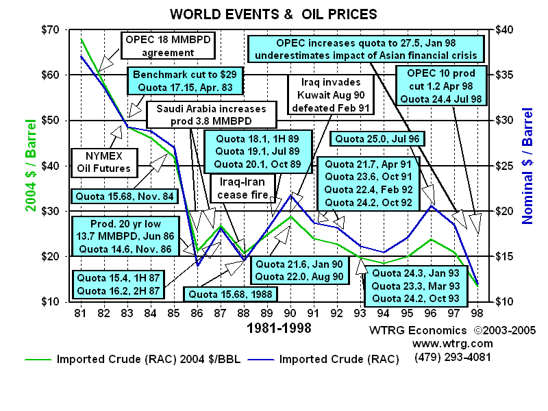World Events and Crude Oil Prices 1981-1998 Click on graph for larger view U.S. Petroleum Consumption Click on graph for larger view Non-OPEC Production & Crude Oil Prices Click on graph for larger view OPEC Production & Crude Oil Prices Click on graph for larger view Russian Crude Oil Production 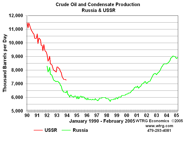Click on graph for larger view
OPEC continued to have mixed success in controlling prices. There were mistakes in timing of quota changes as well as the usual problems in maintaining production discipline among its member countries. The price increases came to a rapid end in 1997 and 1998 when the impact of the economic crisis in Asia was either ignored or severely underestimated by OPEC. In December, 1997 OPEC increased its quota by 2.5 million barrels per day (10 percent) to 27.5 MMBPD effective January 1, 1998. The rapid growth in Asian economies had come to a halt. In 1998 Asian Pacific oil consumption declined for the first time since 1982. The combination of lower consumption and higher OPEC production sent prices into a downward spiral. In response, OPEC cut quotas by 1.25 million b/d in April and another 1.335 million in July. Price continued down through December 1998. Prices began to recover in early 1999 and OPEC reduced production another 1.719 million barrels in April. As usual not all of the quotas were observed but between early 1998 and the middle of 1999 OPEC production dropped by about 3 million barrels per day and was sufficient to move prices above $25 per barrel. With minimal Y2K problems and growing US and world economies the price continued to rise throughout 2000 to a post 1981 high. Between April and October, 2000 three successive OPEC quota increases totaling 3.2 million barrels per day were not able to stem the price increases. Prices finally started down following another quota increase of 500,000 effective November 1, 2000.	World Events and Crude Oil Prices 1997-2003 Click on graph for larger view OPEC Production 1990-2007 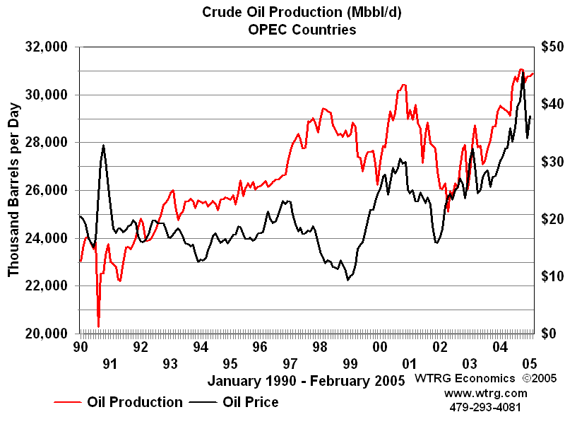Click on graph for larger view
Russian production increases dominated non-OPEC production growth from 2000 forward and was responsible for most of the non-OPEC increase since the turn of the century. Once again it appeared that OPEC overshot the mark. In 2001, a weakened US economy and increases in non-OPEC production put downward pressure on prices. In response OPEC once again entered into a series of reductions in member quotas cutting 3.5 million barrels by September 1, 2001. In the absence of the September 11, 2001 terrorist attack this would have been sufficient to moderate or even reverse the trend. In the wake of the attack crude oil prices plummeted. Spot prices for the U.S. benchmark West Texas Intermediate were down 35 percent by the middle of November. Under normal circumstances a drop in price of this magnitude would have resulted an another round of quota reductions but given the political climate OPEC delayed additional cuts until January 2002. It then reduced its quota by 1.5 million barrels per day and was joined by several non-OPEC producers including Russia who promised combined production cuts of an additional 462,500 barrels. This had the desired effect with oil prices moving into the $25 range by March, 2002. By mid-year the non-OPEC members were restoring their production cuts but prices continued to rise and U.S. inventories reached a 20-year low later in the year. By year end oversupply was not a problem. Problems in Venezuela led to a strike at PDVSA causing Venezuelan production to plummet. In the wake of the strike Venezuela was never able to restore capacity to its previous level and is still about 900,000 barrels per day below its peak capacity of 3.5 million barrels per day. OPEC increased quotas by 2.8 million barrels per day in January and February, 2003. On March 19, 2003, just as some Venezuelan production was beginning to return, military action commenced in Iraq. Meanwhile, inventories remained low in the U.S. and other OECD countries. With an improving economy U.S. demand was increasing and Asian demand for crude oil was growing at a rapid pace. The loss of production capacity in Iraq and Venezuela combined with increased OPEC production to meet growing international demand led to the erosion of excess oil production capacity. In mid 2002, there was over 6 million barrels per day of excess production capacity and by mid-2003 the excess was below 2 million. During much of 2004 and 2005 the spare capacity to produce oil was under a million barrels per day. A million barrels per day is not enough spare capacity to cover an interruption of supply from most OPEC producers. In a world that consumes over 80 million barrels per day of petroleum products that added a significant risk premium to crude oil price and is largely responsible for prices in excess of $40-$50 per barrel. Other major factors contributing to the current level of prices include a weak dollar and the continued rapid growth in Asian economies and their petroleum consumption. The 2005 hurricanes and U.S. refinery problems associated with the conversion from MTBE as an additive to ethanol have contributed to higher prices.	World Events and Crude Oil Prices 2001-2007 Click on graph for larger view Russian Crude Oil Production Click on graph for larger view Venezuelan Oil Production Click on graph for larger view Excess Crude Oil Production Capacity 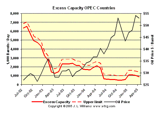Click on graph for larger view
One of the most important factors supporting a high price is the level of petroleum inventories in the U.S. and other consuming countries. Until spare capacity became an issue inventory levels provided an excellent tool for short-term price forecasts. Although not well publicized OPEC has for several years depended on a policy that amounts to world inventory management. Its primary reason for cutting back on production in November, 2006 and again in February, 2007 was concern about growing OECD inventories. Their focus is on total petroleum inventories including crude oil and petroleum products, which are a better indicator of prices that oil inventories alone.
Impact of Prices on Industry Segments Drilling and Exploration
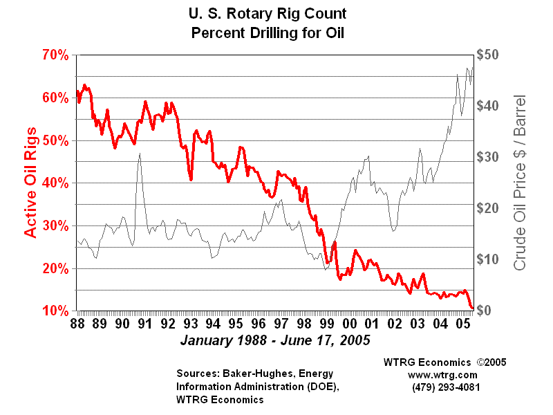
Boom and Bust The Rotary Rig Count is the average number of drilling rigs actively exploring for oil and gas. Drilling an oil or gas well is a capital investment in the expectation of returns from the production and sale of crude oil or natural gas. Rig count is one of the primary measures of the health of the exploration segment of the oil and gas industry. In a very real sense it is a measure of the oil and gas industry's confidence in its own future. At the end of the Arab Oil Embargo in 1974 rig count was below 1500. It rose steadily with regulated crude oil prices to over 2000 in 1979. From 1978 to the beginning of 1981 domestic crude oil prices exploded from a combination of the the rapid growth in world energy prices and deregulation of domestic prices. At that time high prices and forecasts of crude oil prices in excess of $100 per barrel fueled a drilling frenzy. By 1982 the number of rotary rigs running had more than doubled. It is important to note that the peak in drilling occurred over a year after oil prices had entered a steep decline which continued until the 1986 price collapse. The one year lag between crude prices and rig count disappeared in the 1986 price collapse. For the next few years the economy of the towns and cities in the oil patch was characterized by bankruptcy, bank failures and high unemployment.	U.S. Rotary Rig Count 1974-2005 Crude Oil and Natural Gas Drilling 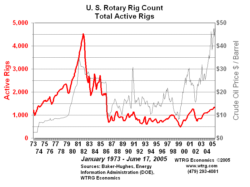Click on graph for larger view
After the Collapse Several trends established were established in the wake of the collapse in crude prices. The lag of over a year for drilling to respond to crude prices is now reduced to a matter of months. (Note that the graph on the right is limited to rigs involved in exploration for crude oil as compared to the previous graph which also included rigs involved in gas exploration.) Like any other industry that goes through hard times the oil business emerged smarter, leaner and more conservative. Industry participants, bankers and investors were far more aware of the risk of price movements. Companies long familiar with accessing geologic, production and management risk added price risk to their decision criteria. Technological improvements were incorporated: Increased use of 3-D seismic data reduced drilling risk. Directional and horizontal drilling led to improved production in many reservoirs. Financial instruments were used to limit exposure to price movements. Increased use of CO2 floods and improved recovery methods to improve production in existing wells. In spite of all of these efforts the percentage of rigs employed in drilling for crude oil decreased from over 60 percent of total rigs at the beginning of 1988 to under 15 percent until a recent resurgence.	U.S. Rotary Rig Count Exploration for Oil 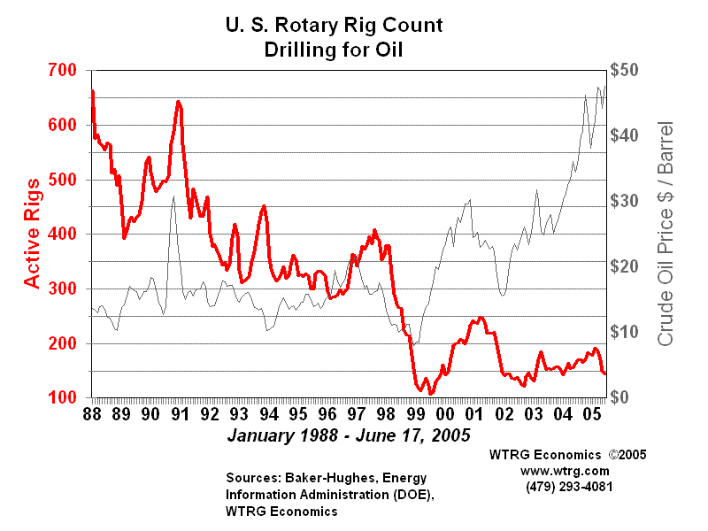Click on graph for larger view U.S. Rotary Rig Count Percent Exploring for Crude Oil Click on graph for larger view
Well Completions - A measure of success? Rig count does not tell the whole story of oil and gas exploration and development. It is certainly a good measure of activity, but it is not a measure of success. After a well is drilled it is either classified as an oil well, natural gas well or dry hole. The percentage of wells completed as oil or gas wells is frequently used as a measure of success. In fact, this percentage is often referred to as the success rate. Immediately after World War II 65 percent of the wells drilled were completed as oil or gas wells. This percentage declined to about 57 percent by the end of the 1960s. It rose steadily during the 1970s to reach 70 percent at the end of that decade. This was followed by a plateau or modest decline through most of the 1980s. Beginning in 1990 shortly after the harsh lessons of the price collapse completion rates increased dramatically to 77 percent. What was the reason for the dramatic increase? For that matter, what was the cause of the steady drop in the 1950s and 1960s or the reversal in the 1970s? Since the percentage completion rates are much lower for the more risky exploratory wells, a shift in emphasis away from development would result in lower overall completion rates. This, however, was not the case. An examination of completion rates for development and exploratory wells shows the same general pattern. The decline was price related as we will explain later. Some would argue that the periods of decline were a result of the fact that every year there is less oil to find. If the industry does not develop better technology and expertise every year, oil and gas completion rates should decline. However, this does will not explain the periods of increase. The increases of the seventies were more related to price than technology. When a well is drilled, the fact that oil or gas is found does not mean that the well will be completed as a producing well. The determining factor is economics. If the well can produce enough oil or gas to cover the additional cost of completion and the ongoing production costs it will be put into production. Otherwise, its a dry hole even if crude oil or natural gas is found. The conclusion is that if real prices are increasing we can expect a higher percentage of successful wells. Conversely if prices are declining the opposite is true. The increases of the 1990s, however, cannot be explained by higher prices. These increases are the result of improved technology and the shift to a higher percentage of natural gas drilling activity. The increased use of and improvements to 3-D seismic data and analysis combined with horizontal and and directional drilling improve prospects for successful completions. The fact that natural gas is easier to see in the seismic data adds to that success rate. Most dramatic is the improvement in the the percentage exploratory wells completed. In the 1990s completion rates for exploratory wells have soared from 25 to 45 percent.	Oil and Gas Well Completion Rates Click on graph for larger view Oil and Gas Well Completion Rates Click on graph for larger view Oil and Gas Well Completion Rates Development Click on graph for larger view U.S. Oil and Gas Well Completion Rates Exploration Click on graph for larger view
Workover Rigs - Maintenance Workover rig count is a measure of the industry's investment in the maintenance of oil and gas wells. The Baker-Hughes workover rig count includes rigs involved in pulling production tubing, sucker rods and pumps from a well that is 1,500 feet or more in depth. Workover rig count is another measure of the health of the oil and gas industry. A disproportionate percentage of workovers are associated with oil wells. Workover rigs are used to pull tubing for repair or replacement of rods, pumps and tubular goods which are subject to wear and corrosion. A low level of workover activity is particularly worrisome because it is indicative of deferred maintenance. The situation is similar to the aging apartment building that no longer justifies major renovations and is milked as long as it produces a positive cash flow. When operators are in a weak cash position workovers are delayed as long as possible. Workover activity impacts manufacturers of tubing, rods and pumps. Service companies coating pipe and other tubular goods are heavily affected.	U.S. Workover Rigs and Crude Oil Prices Click on graph for larger view
[WTRG's HOME PAGE] Copyright 1996-2007 by James L. Williams

some index

notes for index.
generally, people like to quote the index, but to explain them. some index explanation. FYI

EXPLANATORY NOTES
CENTRAL BANKS
Federal Reserve
TAFs: The Term Auction Facilities (TAFs) were introduced by the Fed on 12 Dec 2007 to get around the stigma banks associated with accessing the
Discount Window. They are normally auctions of one-month money with a minimum bid rate set by the prevailing 1M OIS and use the same collateral
requirements of the Discount Window (incl. ABCP, CDOs etc). Recently, the Fed also introduced longer dated auctions for 84-day money.
TSLF: Under the Term Securities Lending Facility (TSLF) the Fed lends Treasury securities to primary dealers for 28 days in exchange for other
securities. The range of acceptable securities was widened in mid-September to include all investment grade debt. In addition, the frequency and the
size of the operations were increased.
Expanded OMOs: On Mar 7, the Fed introduced a new type of 28-day term repurchase transactions in addition to its regular operations. These
repos are virtually identical to the Fed's normal open market operations (OMOs) in terms of collateral requirements and are open to primary dealers
only. It is noticeable that the bid/cover ratios for the OMOs are higher than that for the TAFs even though both are basically auctions for 28-day cash.
The explanation for this probably lies in the fact that the TAFs are only open to depository institutions while the OMOs are only open to primary
dealers (mainly investment banks) and the latter group have the more constrained balance sheets at the moment.
ECB
The ECB's Open Market Operations are shown as a proportion of 'autonomous factors' (structural demand for funds) and minimum reserve
requirements. This filters out changes in liquidity provision due to time-varying changes in demand or changes in reserve requirements. As a result,
the ratio typically reverts to 100% at month-end. The amount of USD liquidity provided under the FX swap agreement concluded with the Fed in Dec
07 and widened later is also shown.
BoE
The chart shows the secured overnight rate which is the rate on overnight gilt repos. Spikes in the rate over Bank Rate indicate short term funding
pressures in the sterling market. We also show the amount of USD liqudity provided under an FX swap agreement with the Fed from Sep 08.
MONEY MARKETS
TED spread: The 3M Libor rate over the 3M T-bill rate. This spread gives an indication of the interbank risk premium as it filters out the risk-free
Treasury rate.
3M Libor over OIS: 3-month rates are the Libors in the respective currency. The Overnight Indexed Swap is an interest rate swap with the fixed leg
the quoted rate and the floating leg computed using a published overnight rate. The floating leg for the USD OIS is the Effective Fed Funds rate while
for GBP it is SONIA and for EUR it is EONIA. It is therefore a useful although not precise indicator of market expectations of future policy rates.
Commercial Paper Outstanding: The chart indicates the stock of outstanding ABCP and unsecured CP in the US. The data is updated on a weekly
basis (Thu).
US Commercial Paper Yields: Yields on Top Tier (A1+/P1/F1+) US Commercial Paper based on a composite index published by Bloomberg.
CREDIT
High grade credit default swap index: The European index is the 5yr iTraxx High Grade index which is composed of 125 investment grade entities,
distributed among nine sectors. The index is expressed in basis points. The US index is the CDX North America Investment Grade Index published
by Markit, which is composed of 125 entities, distributed over six sectors and expressed in bps.
30yr Mortgage Rate: US Home Mortgage 30 yr fixed, national average, with a one-day delay from bankrate.com
ABX: The ABX index is a synthetic index comprising of 20 equally weighted constituents of ABS in 5 rating categories (AAA, AA, A, BBB, BBB-). The
ABS themselves reference Home Equity Loans (HEL) with a minimum deal size of $500mn and an average life of between 4-6 years. Hence, the
index has been used considerably in the past in an attempt to hedge exposures on subprime loans. The ABX index trades on the basis of price rather
than spread, as the possibility of prepayment on the loans makes it difficult to devise accurate duration estimates.
Emerging Markets: The Global Emerging Market Sovereign Bond Index (ESBI) is a proprietary Citi index. We show it expressed as an optionadjusted
spread over US Treasuries. The MSCI Emerging Markets Equity Index is a local currency index of global emerging markets.
OTHER
Crude oil: shows the generic 1-month rolling contract of WTI as published by Bloomberg.
Gold: is the spot price of gold in USD/Oz.
Citi Economic Surprise Index: The Citigroup ESIs are weighted historical standard deviations of data surprises (actual releases vs Bloomberg
survery median). A positive reading of the Economic Surprise Index suggests that economic releases have on balance been beating consensus. The
indices are calculated daily in a rolling three-month window. The weights of economic indicators are derived from relative high-frequency spot FX
impacts of 1 standard deviation data surprises. The indices also employ a time decay function to replicate the limited memory of markets. They can
be accessed on Bloomberg via GO.
VIX: The CBOE's Volatility Index reflects a market estimate of future volatility, based on the weighted average of the implied volatilities for a wide
range of strikes. 1st and 2nd month expirations are used until 8 days from expiration, then the 2nd and 3rd are used.
S&P 500: is a capitalisation-weighted index of 500 stocks. The index is designed to measure performance of the broad domestic US economy
through changes in the aggreate market value of 500 stocks representing all major industries.
S&P 500 Financials Index: is a market cap-weighted index consisting of the 90 biggest financial stocks in the US